In software engineering, efficiency is not a luxury; it is a requirement. As systems scale, the difference between an efficient algorithm and an inefficient one can mean the difference between a responsive application and a complete system failure. To measure this efficiency, we use Big O Notation.
The Theory: Big O, Omega, and Theta
To formally analyze algorithms, we use asymptotic notation. While most technical interviews focus on Big O, it is important to understand the broader context.
- Big O (O): Represents the upper bound. It describes the worst-case scenario.
- Big Omega (Ω): Represents the lower bound. It describes the best-case scenario.
- Big Theta (Θ): Represents the tight bound. It describes the average or exact rate of growth.
In practice, we design for the worst case (Big O) because it provides a guarantee that the software will never perform worse than a certain limit.
Time Complexity Classes
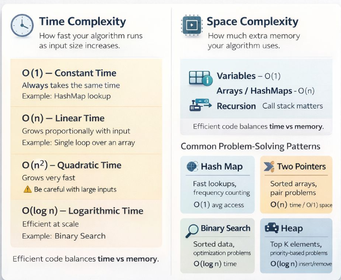
Time complexity measures how the execution time of an algorithm increases relative to the size of the input (n).
O(1) — Constant Time
The execution time remains the same regardless of the input size. This is the ultimate goal for
optimization.
Example: Accessing an element in an array by index or a lookup in a HashMap.
O(log n) — Logarithmic Time
The execution time grows logarithmically. Typically seen in algorithms that divide the problem in half
during each step.
Example: Binary Search.
O(n) — Linear Time
The execution time grows proportionally with the input size.
Example: A single loop iterating through an array of size n.
O(n log n) — Linearithmic Time
Common in efficient sorting algorithms. It involves performing a logarithmic operation n times.
Example: Merge Sort, Quick Sort.
O(n²) — Quadratic Time
The execution time grows with the square of the input size. Often the result of nested loops over the
same data set.
Example: Bubble Sort, checking all pairs in an array.
Space Complexity: The Hidden Cost
Space complexity measures the total amount of extra memory an algorithm uses relative to the input size. In modern systems, we often trade space for time (e.g., using a HashMap to speed up lookups).
- O(1) Space: No extra memory is used regardless of input size (e.g., simple counters or pointers).
- O(n) Space: Extra memory grows linearly with the input (e.g., creating a copy of an array or storing elements in a Set).
- Recursion: Each recursive call adds a frame to the call stack. A recursive function with depth d has at least O(d) space complexity.
Common Problem-Solving Patterns
To optimize complexity, we rely on established patterns that have known performance characteristics.
Two Pointers
Works on sorted data. Reduces O(n²) search to O(n) by moving markers from both ends or at different speeds.
Sliding Window
Optimizes subarray/substring problems. Avoids recomputation by "sliding" a range over the data in O(n) time.
Frequency Counting
Uses a Hash Map to store occurrences. Great for reducing repeated scans and identifying patterns in O(n) time.
Binary Search
Requires sorted input. Dramatically cuts the search space in half each time, achieving O(log n).
Conclusion
The goal of performance analysis is not to guess but to design with intention. By understanding the complexity of your operations, you can build systems that are not only functional but truly scalable. Master the patterns, analyze the bottlenecks, and design for the future.